University of Tehran

We shall see how simulation can be used to compare alternative ordering policies for an inventory system. Many of the elements of our model are representative of those found in actual inventory systems.

A company that sells a single product would like to decide how many items it should have in inventory for each of the next n months (n is a fi xed input parameter). The times between demands are IID exponential random variables with a mean of 0.1 month. The sizes of the demands, D, are IID random variables (independent of when the demands occur), with

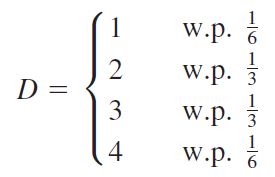
where w.p. is read “with probability.”

At the beginning of each month, the company reviews the inventory level and decides how many items to order from its supplier. If the company orders Z items, it incurs a cost of K + iZ, where K = $32 is the setup cost and i = $3 is the incremental cost per item ordered. (If Z = 0, no cost is incurred.) When an order is placed, the time required for it to arrive (called the delivery lag or lead time) is a random variable that is distributed uniformly between 0.5 and 1 month.

The company uses a stationary (s, S) policy to decide how much to order, i.e.,

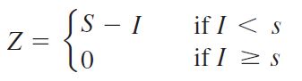
where I is the inventory level at the beginning of the month.

When a demand occurs, it is satisfi ed immediately if the inventory level is at least as large as the demand. If the demand exceeds the inventory level, the excess of demand over supply is backlogged and satisfi ed by future deliveries. (In this case, the new inventory level is equal to the old inventory level minus the demand size, resulting in a negative inventory level.) When an order arrives, it is fi rst used to eliminate as much of the backlog (if any) as possible; the remainder of the order (if any) is added to the inventory.

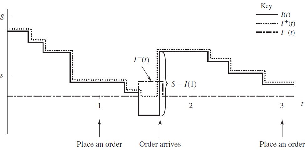
So far, we have discussed only one type of cost incurred by the inventory system, the ordering cost. However, most real inventory systems also have two additional types of costs, holding and shortage costs, which we discuss after introducing some additional notation. Let I(t) be the inventory level at time t [note that I(t) could be positive, negative, or zero]; let I+(t) = max{I(t), 0} be the number of items physically on hand in the inventory at time t [note that I+(t) > 0]; and

let I-(t) = max{-I(t), 0} be the backlog at time t [I-(t) > 0 as well].

For our model, we shall assume that the company incurs a holding cost of h = $1 per item per month held in (positive) inventory. The holding cost includes such costs as warehouse rental, insurance, taxes, and maintenance, as well as the opportunity cost of having capital tied up in inventory rather than invested elsewhere. We have ignored in our formulation the fact that some holding costs are still incurred when I+(t) = 0.

See Results

Programming Language: Python

Course: Performance Evolution of Computer Systems Course